import matplotlib.pyplot as plt

import numpy as np # need for log() function
import pandas as pd
import collections
from collections import CounterExploring Texts using the Vector Space Model
Text and code copied from:
Karsdorp, F., Kestemont, M., & Riddell, A. (2021). Humanities Data Analysis: Case Studies with Python, Princeton University Press.
Adapted by Eliese-Sophia Lincke & Shai Gordin for the purposes of the course Ancient Language Processing (summer term 2024)
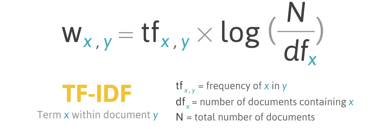
From Texts to Vectors: TF-IDF
When using the vector space model, a corpus—a collection of documents, each represented as a bag of words—is typically represented as a matrix, in which each row represents a document from the collection, each column represents a word from the collection’s vocabulary, and each cell represents the frequency with which a particular word occurs in a document.
A matrix arranged in this way is often called a document-term matrix—or term-document matrix where: * rows are associated with documents * word counts are in the columns.
```{table} Example of a vector space representation with four documents (rows) and a vocabulary of four words (columns). For each document the table lists how often each vocabulary item occurs.
| roi | ange | sang | perdu | |
|---|---|---|---|---|
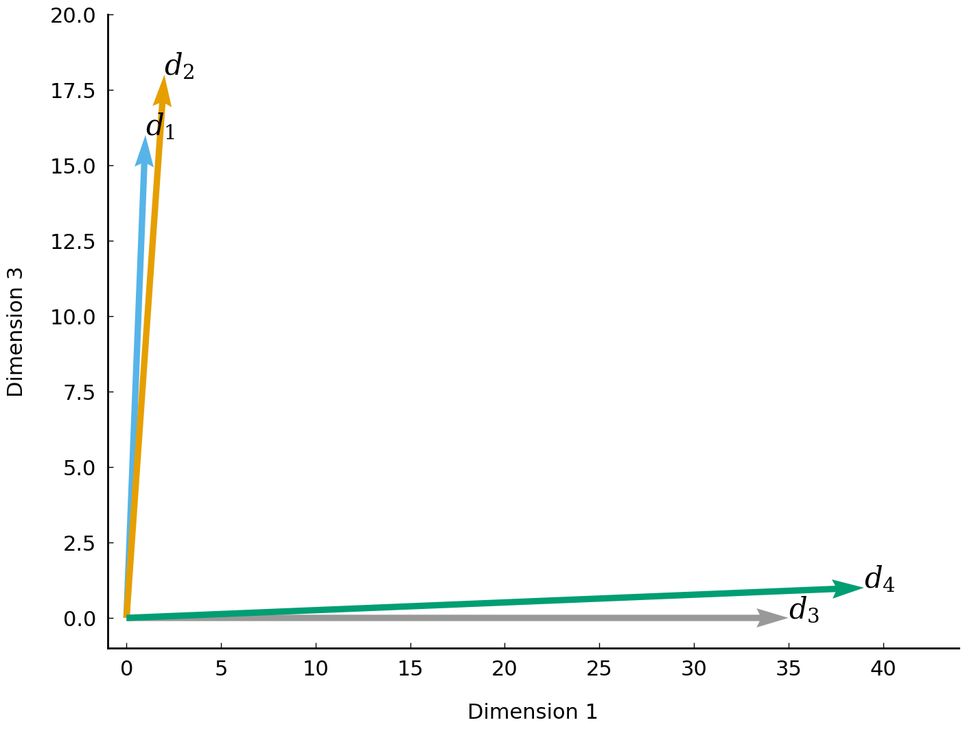
| \(d_1\) | 1 | 2 | 16 | 21 |
| \(d_2\) | 2 | 2 | 18 | 19 |
| \(d_3\) | 35 | 41 | 0 | 2 |
| \(d_4\) | 39 | 55 | 1 | 0 |
In this table, each document $d_i$ is represented as a vector, which, essentially, is a list of numbers---word frequencies in our present case. A <span class="index">vector space</span> is nothing more than a collection of numerical vectors, which may, for instance, be added together and multiplied by a number. Documents represented in this manner may be compared in terms of their *coordinates* (or *components*). For example, by comparing the four documents on the basis of the second coordinate, we observe that the first two documents ($d_1$ and $d_2$) have similar counts, which might be an indication that these two documents are somehow more similar. To obtain a more accurate and complete picture of document similarity, we would like to be able to compare documents more holistically, using *all* their components. In our example, each document represents a point in a four-dimensional vector space. We might hypothesize that similar documents use similar words, and hence reside close to each other in this space. To illustrate this, we demonstrate how to visualize the documents in space using the first and third components.
* TF-IDF: Concept

* TF-IDF: Simple calculation
### Preprocessing
::: {.cell}
``` {.python .cell-code}
# raw data
akk05 = ['ana', 'eššūtu', 'kašāru', 'mātu', 'Aššur', 'ana', 'UNK', 'ālu', 'epēšu', 'ēkallu', 'mūšabu', 'šarrūtu', 'ina', 'libbu', 'nadû', 'UNK', 'šumu', 'nabû', 'kakku', 'Aššur', 'bēlu', 'ina', 'libbu', 'ramû', 'nišu', 'mātu', 'kišittu', 'qātu', 'ina', 'libbu', 'wašābu', 'biltu', 'maddattu', 'kânu', 'itti', 'nišu', 'mātu', 'Aššur', 'manû', 'ṣalmu', 'šarrūtu', 'u', 'ṣalmu', 'ilu', 'rabû', 'bēlu', 'epēšu', 'lītu', 'u', 'danānu', 'ša', 'ina', 'zikru', 'Aššur', 'bēlu', 'eli', 'mātu', 'šakānu', 'ina', 'muhhu', 'šaṭāru', 'ina', 'UNK', 'izuzzu', 'UNK', 'UNK', 'biltu', 'hurāṣu', 'ina', 'dannu', 'UNK', 'līm', 'biltu', 'kaspu', 'UNK', 'maddattu', 'mahāru', 'ina', 'UNK', 'palû', 'Aššur', 'bēlu', 'takālu', 'ana', 'Namri', 'UNK', 'Bit-Zatti', 'Bit-Abdadani', 'Bit-Sangibuti', 'UNK', 'alāku', 'UNK', 'akāmu', 'gerru', 'amāru', 'Nikkur', 'ālu', 'dannūtu', 'wašāru', 'UNK', 'zanānu', 'Nikkurayu', 'kakku', 'UNK', 'sisû', 'parû', 'alpu', 'UNK', 'Sassiašu', 'Tutašdi', 'UNK']
akk08 = ['UNK', 'nišu', 'ana', 'mātu', 'Aššur', 'warû', 'UNK', 'UNK', 'ina', 'UNK', 'palû', 'Aššur', 'bēlu', 'takālu', 'UNK', 'UNK', 'UNK', 'UNK', 'UNK', 'UNK', 'UNK', 'UNK', 'UNK', 'UNK', 'UNK', 'UNK', 'Sulumal', 'Meliddayu', 'Tarhu-lara', 'Gurgumayu', 'UNK', 'UNK', 'UNK', 'mātitān', 'ana', 'emūqu', 'ahāmiš', 'takālu', 'UNK', 'UNK', 'ina', 'lītu', 'u', 'danānu', 'ša', 'Aššur', 'bēlu', 'itti', 'mahāṣu', 'dīktu', 'dâku', 'UNK', 'UNK', 'qurādu', 'dâku', 'hurru', 'natbāku', 'šadû', 'malû', 'narkabtu', 'UNK', 'UNK', 'ana', 'lā', 'mānu', 'leqû', 'ina', 'qablu', 'tidūku', 'ša', 'Ištar-duri', 'UNK', 'UNK', 'UNK', 'UNK', 'ina', 'qātu', 'ṣabātu', 'UNK', 'līm', 'UNK', 'līm', 'UNK', 'meʾatu', 'UNK', 'UNK', 'UNK', 'UNK', 'ištu', 'UNK', 'UNK', 'Ištar-duri', 'ana', 'ezēbu', 'napištu', 'mūšiš', 'halāqu', 'lāma', 'šamšu', 'urruhiš', 'naprušu', 'UNK', 'UNK', 'itti', 'šiltāhu', 'pāriʾu', 'napištu', 'adi', 'titūru', 'Purattu', 'miṣru', 'mātu', 'ṭarādu', 'eršu', 'UNK', 'UNK', 'ša', 'šadādu', 'šarrūtu', 'kunukku', 'kišādu', 'adi', 'abnu', 'kišādu', 'narkabtu', 'šarrūtu', 'UNK', 'UNK', 'mimma', 'šumu', 'mādu', 'ša', 'nību', 'lā', 'išû', 'ekēmu', 'sisû', 'UNK', 'UNK', 'ummiānu', 'ana', 'lā', 'mānu', 'leqû', 'bītu', 'ṣēru', 'kuštāru', 'šarrūtu', 'UNK', 'UNK', 'unūtu', 'tāhāzu', 'mādu', 'ina', 'qerbu', 'ušmannu', 'ina', 'išātu', 'šarāpu', 'UNK', 'UNK', 'UNK', 'eršu', 'ana', 'Ištar', 'šarratu', 'Ninua', 'qiāšu', 'UNK']
akk11 = ['mašku', 'pīru', 'šinnu', 'pīru', 'argamannu', 'takiltu', 'lubuštu', 'birmu', 'kitû', 'lubuštu', 'mātu', 'mādu', 'UNK', 'UNK', 'UNK', 'UNK', 'UNK', 'UNK', 'tillu', 'pilaqqu', 'UNK', 'UNK', 'UNK', 'UNK', 'ina', 'qerbu', 'Arpadda', 'mahāru', 'Tutammu', 'šarru', 'Unqi', 'ina', 'adû', 'ilu', 'rabû', 'haṭû', 'šiāṭu', 'napištu', 'gerru', 'UNK', 'lā', 'malāku', 'itti', 'ina', 'uzzu', 'libbu', 'UNK', 'ša', 'Tutammu', 'adi', 'rabû', 'UNK', 'Kunalua', 'ālu', 'šarrūtu', 'kašādu', 'nišu', 'adi', 'maršītu', 'UNK', 'kūdanu', 'ina', 'qerbu', 'ummānu', 'kīma', 'ṣēnu', 'manû', 'UNK', 'ina', 'qabaltu', 'ēkallu', 'ša', 'Tutammu', 'kussû', 'nadû', 'UNK', 'UNK', 'UNK', 'UNK', 'UNK', 'meʾatu', 'biltu', 'kaspu', 'ina', 'dannu', 'UNK', 'meʾatu', 'biltu', 'UNK', 'UNK', 'unūtu', 'tāhāzu', 'lubuštu', 'birmu', 'kitû', 'rīqu', 'kalāma', 'būšu', 'ēkallu', 'UNK', 'Kunalua', 'ana', 'eššūtu', 'ṣabātu', 'Unqi', 'ana', 'pāṭu', 'gimru', 'kanāšu', 'UNK', 'šūt', 'rēšu', 'bēlu', 'pīhātu', 'eli', 'šakānu']
akk13 = ['UNK', 'ana', 'Hatti', 'adi', 'mahru', 'wabālu', 'šūt', 'rēšu', 'šaknu', 'mātu', 'Naʾiri', 'Supurgillu', 'UNK', 'adi', 'ālu', 'ša', 'liwītu', 'kašādu', 'šallatu', 'šalālu', 'Šiqila', 'rabû', 'birtu', 'UNK', 'šalālu', 'ana', 'Hatti', 'adi', 'mahru', 'wabālu', 'UNK', 'meʾatu', 'šallatu', 'Amlate', 'ša', 'Damunu', 'UNK', 'līm', 'UNK', 'meʾatu', 'šallatu', 'Deri', 'ina', 'Kunalua', 'UNK', 'Huzarra', 'Taʾe', 'Tarmanazi', 'Kulmadara', 'Hatatirra', 'Irgillu', 'ālu', 'ša', 'Unqi', 'wašābu', 'UNK', 'šallatu', 'Qutu', 'Bit-Sangibuti', 'UNK', 'līm', 'UNK', 'meʾatu', 'Illilayu', 'UNK', 'līm', 'UNK', 'meʾatu', 'UNK', 'Nakkabayu', 'Budayu', 'ina', 'UNK', 'Ṣimirra', 'Arqa', 'Usnu', 'Siʾannu', 'ša', 'šiddu', 'tiāmtu', 'wašābu', 'UNK', 'meʾatu', 'UNK', 'Budayu', 'Dunu', 'UNK', 'UNK', 'UNK', 'UNK', 'meʾatu', 'UNK', 'Belayu', 'UNK', 'meʾatu', 'UNK', 'Banitayu', 'UNK', 'meʾatu', 'UNK', 'Palil-andil-mati', 'UNK', 'meʾatu', 'UNK', 'Sangillu', 'UNK', 'Illilayu', 'UNK', 'meʾatu', 'UNK', 'šallatu', 'Qutu', 'Bit-Sangibuti', 'ina', 'pīhātu', 'Tuʾimmu', 'wašābu', 'UNK', 'meʾatu', 'UNK', 'šallatu', 'Qutu', 'Bit-Sangibuti', 'ina', 'Til-karme', 'wašābu', 'itti', 'nišu', 'mātu', 'Aššur', 'manû', 'ilku', 'tupšikku', 'kī', 'ša', 'Aššuru', 'emēdu', 'maddattu', 'ša', 'Kuštašpi', 'Kummuhayu', 'Rahianu', 'Ša-imerišayu', 'Menaheme', 'Samerinayu', 'Hi-rumu', 'Ṣurrayu', 'Sibitti-Biʾil', 'Gublayu', 'Uriaikki', 'Quayu', 'Pisiris', 'Gargamišayu', 'Eni-il', 'Hamatayu', 'Panammu', 'Samʾallayu', 'Tarhu-lara', 'Gurgumayu', 'Sulumal', 'Meliddayu', 'Dadilu']:::
# returns a list of lists, each lists is one document in the corpus

tokenized_corpus = []
for doc in [akk05, akk08, akk11, akk13] :
  akk = []
  for token in doc :
    akk.append(token)#.lower())
  tokenized_corpus.append(akk)

for doc in tokenized_corpus :
  print(doc)
Counter implements a number of methods specialized for convenient and rapid tallies. For instance, the method Counter.most_common returns the n most frequent items:
# Count token frequencies

vocabulary_akk = Counter(akk05)
print(vocabulary_akk)
print(vocabulary_akk.most_common(n=5))
Calculations of the components
Extract a vocabulary (the inventory of types/lemmata) from a corpus
- Arguments:
tokenized_corpus(list): a tokenized corpus represented, list of lists of strings.min_count(int, optional): the minimum occurrence count of a vocabulary item in the corpus.max_count(int, optional): the maximum occurrence count of a vocabulary item in the corpus. Note that the default maximum count is set to infinity (max_count=float(‘inf’)). This ensures that none of the high-frequency words are filtered without further specification.
- Returns:
list: an alphabetically ordered list of unique words in the corpus
def extract_vocabulary(tokenized_corpus, min_count=1, max_count=float('inf')):

    vocabulary = collections.Counter()
    for document in tokenized_corpus:
        vocabulary.update(document)
    vocabulary = {word for word, count in vocabulary.items()
                  if count >= min_count and count <= max_count}
    return sorted(vocabulary)
# Call the function
vocabulary = extract_vocabulary(tokenized_corpus, min_count = 1)
print(vocabulary)# Check token counts for each type in the vocabulary
bags_of_words = []
for document in tokenized_corpus:
tokens = [word for word in document if word in vocabulary]
bags_of_words.append(collections.Counter(tokens))
#bags_of_words.extend(collections.Counter(tokens))
for count in bags_of_words :
print(count)
#print(bags_of_words)Calculate the term frequency (TF)
Transform a tokenized corpus into a document-term matrix.
- Arguments:
tokenized_corpus(list): a tokenized corpus as a list of lists of strings.vocabulary(list): A list of unique words (types).
- Returns:
list: A list of lists representing the frequency of each term invocabularyfor each document in the corpus.
## Calculate term frequency (TF)
# raw count

def corpus2dtm_raw(tokenized_corpus, vocabulary):

    document_term_matrix = []
    for document in tokenized_corpus:
        document_counts = collections.Counter(document)
        row = [document_counts[word] for word in vocabulary]
        document_term_matrix.append(row)
    return document_term_matrix
# Call the function
document_term_matrix = corpus2dtm_raw(tokenized_corpus, vocabulary)
print(document_term_matrix)
# Convert result into a dataframe
tf_df_abs = pd.DataFrame(document_term_matrix, columns=vocabulary)
tf_df_absThere are three (and possibly more) ways to calculate the TF: * raw count (token count) – like in the function above
This is the simplest form, where TF is just the raw count of the term in the document:
TF(t,d) = count of term t in document d * relative frequency (token count / number of tokens in the document)
TF is normalized by dividing the raw count by the total number of terms in the document:
TF(t,d) = count of term t in document d / total number of tokens in document d * logarithmically scaled: typically involves a normalization step to account for the length of the document. This reduces the impact of (very) frequent terms.
TF(t,d) = log(count of term t in document d + 1)
(When the term frequency is 0, + 1 avoids log(0) which would result in an error.)
# Demonstration of different calculations of the term frequency

def raw_count_tf(term, document):
    return document.count(term)

def relative_frequency_tf(term, document):
    term_count = document.count(term)
    total_terms = len(document)
    return term_count / total_terms if total_terms > 0 else 0 # avoid division by 0

def log_scaled_tf(term, document):
    total_terms = len(document)
    term_count = document.count(term)
    return np.log(1 + term_count) # avoid log(0) by adding 1

# Example document
document = ["this", "is", "a", "sample", "document", "document", "is", "a", "sample", "sample", "sample", "sample", "sample", "sample"]

term = "sample" # change to "sample" to see the scaling down effect for frequent terms

print("Raw Count TF:", raw_count_tf(term, document))
print("Relative Frequency TF:", relative_frequency_tf(term, document))
print("Log Scaled TF:", log_scaled_tf(term, document)) # natural base of logarithm (e = "Euler's number")
## Calculate term frequency (TF) for our corpus
# relative frequency
def corpus_tf(tokenized_corpus, vocabulary):
document_term_matrix = []
for document in tokenized_corpus:
term_per_document_counts = collections.Counter(document)
total_terms = sum(term_per_document_counts.values())
#total_terms = len(document_counts)
#row = [term_per_document_counts[word] for word in vocabulary]
row = [np.log(1 + term_per_document_counts[word]) for word in vocabulary]
document_term_matrix.append(row)
return document_term_matrix# Call the function
# Calculate term frequency (TF) document-term matrix
term_frequency_matrix = corpus_tf(tokenized_corpus, vocabulary)
# Convert the matrix to a DataFrame for easier visualization
tf_df_log = pd.DataFrame(term_frequency_matrix, columns=vocabulary)
tf_df_log#["libbu"]Calculate the Inverse Document Frequency (IDF)
- N = number of documents (in the corpus)
- df_term_counts = number of documents which contain term t
- absolute
IDF(t) = number of documents / number of documents containing term t - logarithmic
IDF(t) = log(number of documents / number of documents containing term t + 1)
# Step 1: Calculate the total number of documents (N): How many documents are there in the corpus?
N = len(tf_df_abs)
print(N)

# Step 2: Calculate the document frequency (DF) for each term: In how many documents does the term appear?
df_nonzero = tf_df_abs > 0  # Convert counts to binary (True/False)
#print(df_nonzero)
df_term_counts = df_nonzero.sum(axis=0)  # Sum across rows, i.e. across documents; rows/documents set to 'False' are not counted
print(df_term_counts)

# Step 3: Calculate the IDF for each term
# add 1 for normalization
idf = np.log(N / (df_term_counts + 1 )) + 1 # natural base ("Euler's number")

# Display the IDF values
idf_df = pd.DataFrame(idf, columns=['IDF']).T
idf_df.loc['df_term_count'] = df_term_counts
idf_df#.iloc[:, 90:105]
Putting it all together: the TF-IDF
Simple TF-IDF
Multiply term frequency and inverse document frequency
# Perform element-wise multiplication
tf_idf_df = tf_df_log * idf_df.loc['IDF']

#tf_idf_df.iloc[:, 90:105]
tf_idf_df#["libbu"]
Weighted TF-IDF
def calculate_tf_weighted(term, document):
    term_count = document.count(term)
    if term_count > 0:
        tf = 1 + np.log(term_count)
    else:
        tf = 0
    return tf

def calculate_idf_weighted(term, corpus):
    num_documents_with_term = sum(1 for doc in corpus if term in doc)
    idf = np.log((len(corpus) + 1) / (num_documents_with_term + 1)) + 1
    return idf

def calculate_tf_idf_weighted(term, document, corpus):
    tf = calculate_tf_weighted(term, document)
    idf = calculate_idf_weighted(term, corpus)
    tf_idf = tf * idf
    return tf_idf

# Define a function to calculate the weighted TF-IDF for every document in the corpus
def calculate_tf_idf_matrix(tokenized_corpus, vocabulary):
    tf_idf_matrix = []
    for document in tokenized_corpus:
        row = [calculate_tf_idf_weighted(term, document, tokenized_corpus) for term in vocabulary]
        tf_idf_matrix.append(row)
    return tf_idf_matrix
#Calculate the TF-IDF weighted matrix for the entire corpus
tf_idf_matrix = calculate_tf_idf_matrix(tokenized_corpus, vocabulary)
# Step 3: Convert the matrix to a DataFrame
tf_idf_df = pd.DataFrame(tf_idf_matrix, columns=vocabulary)
# Display the resulting TF-IDF DataFrame
tf_idf_df#["Aššur"]#["libbu"]Predefined TF-IDF functions from scikit-learn
In the main code of the course, we will use a predefined function from the machine learning library scikit-learn.
Learn more about the weighting and normalization in scikit-learns TF-IDF calculations,
cf. in particular the “Numeric example of a tf-idf matrix”
TfidfVectorizer requires a list of strings as input. Each string is an entire text (document).
## Alternative preprocessing for the TfidfVectorizer from SciKitLearn
# returns a list of strings, each string is one document

tokenized_corpus_asStr = []
for doc in [akk05, akk08, akk11, akk13] :
  akk = ""
  for token in doc :
    akk = akk + token + " "
  tokenized_corpus_asStr.append(akk.strip())

for doc in tokenized_corpus_asStr :
  print(doc + " ------")
#print(tokenized_corpus_asStr)
from sklearn.feature_extraction.text import TfidfVectorizer
#from sklearn.feature_extraction.text import TfidfTransformer
# Step 1: Instantiate TfidfVectorizer
vectorizer = TfidfVectorizer(min_df = 0, max_df = 100, norm = "l1") # with and without normalization (norm = None)
# Step 2: Fit and transform the corpus
tfidf_matrix = vectorizer.fit_transform(tokenized_corpus_asStr)
# Display the TF-IDF matrix
#tfidf_matrix.toarray()
tfidf_df = pd.DataFrame(tfidf_matrix.toarray(), columns=vectorizer.get_feature_names_out())
tfidf_df#["aššur"]#["libbu"]
# Display the feature names
#vectorizer.get_feature_names_out()