Interpretable shape features and diplomatic genealogies
Paper section: Results §3.3 · Notebooks:2.4, 10, 10.1, 11, 11.1
Overview
A Variational Autoencoder (VAE) with a 12-dimensional bottleneck compresses each tablet’s 80×80 binary silhouette into a structured 12-number vector. Unlike pixel ratios or classification labels, these 12 coordinates form a continuous geometric space in which similar tablet shapes cluster together and morphological transitions can be traced as paths.
Two key questions drive this analysis:
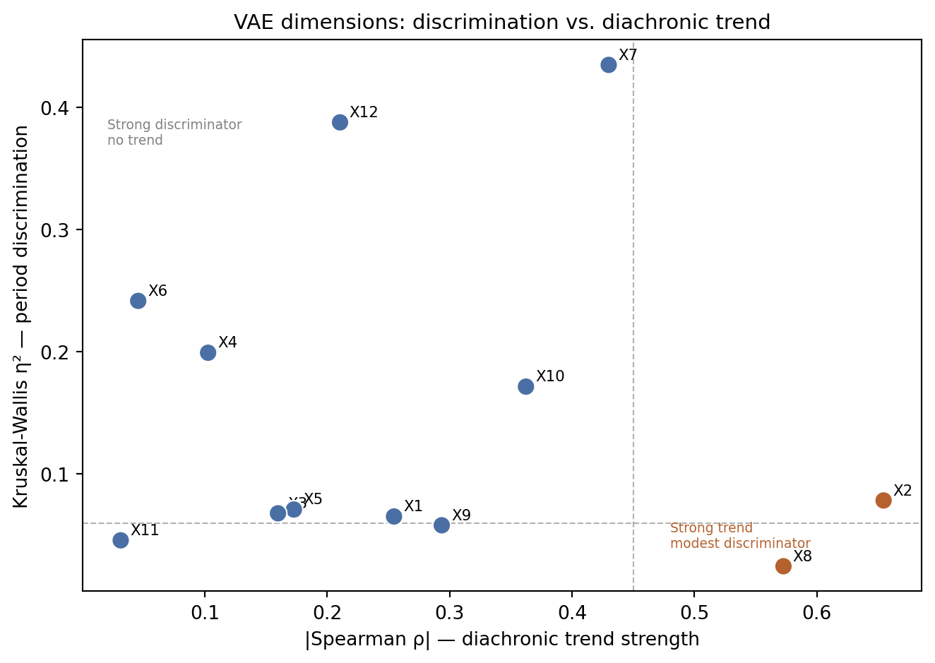
Which dimensions best discriminate between historical periods?
Which dimensions best track the diachronic trend across time?
The answer to these questions is the same for no single dimension — and that dissociation is itself the finding.
Discrimination vs. trend: the core result
Code
import pandas as pd, matplotlib.pyplot as plt, numpy as npdf = pd.read_csv("../../paper/figures/vae_dim_stats.csv")fig, ax = plt.subplots(figsize=(7, 5))colors = ['#b5622e'if s =='**'else'#4a6fa5'for s in df['sig']]ax.scatter(df['abs_rho'], df['eta2'], c=colors, s=90, zorder=5, edgecolors='white', lw=0.8)for _, row in df.iterrows(): ax.annotate(row['Dimension'], (row['abs_rho'], row['eta2']), xytext=(5, 3), textcoords='offset points', fontsize=8)ax.axhline(0.06, color='grey', ls='--', lw=0.8, alpha=0.6)ax.axvline(0.45, color='grey', ls='--', lw=0.8, alpha=0.6)ax.set_xlabel("|Spearman ρ| — diachronic trend strength", fontsize=10)ax.set_ylabel("Kruskal-Wallis η² — period discrimination", fontsize=10)ax.set_title("VAE dimensions: discrimination vs. diachronic trend", fontsize=11)ax.text(0.02, 0.37, 'Strong discriminator\nno trend', fontsize=7, color='grey')ax.text(0.48, 0.04, 'Strong trend\nmodest discriminator', fontsize=7, color='#b5622e')plt.tight_layout()plt.show()
Figure 1: Kruskal-Wallis η² (period discrimination power, y-axis) vs. Spearman |ρ| (diachronic trend strength, x-axis) for all 12 VAE dimensions. Significant trend dimensions (p < 0.05) shown in red.
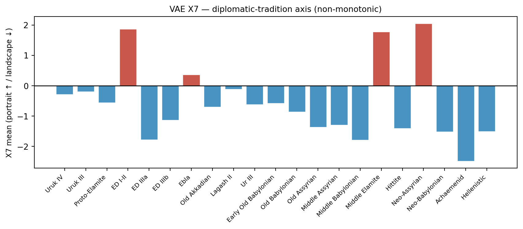
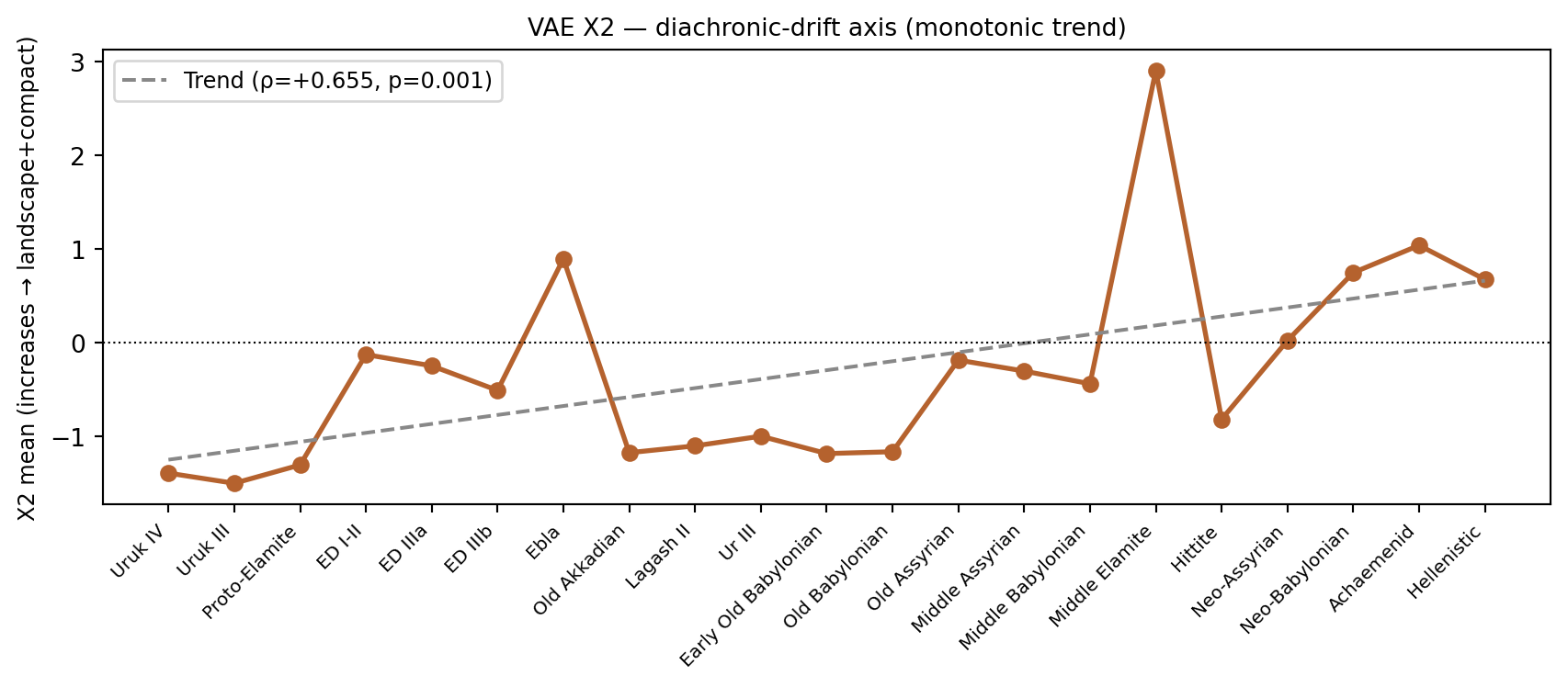
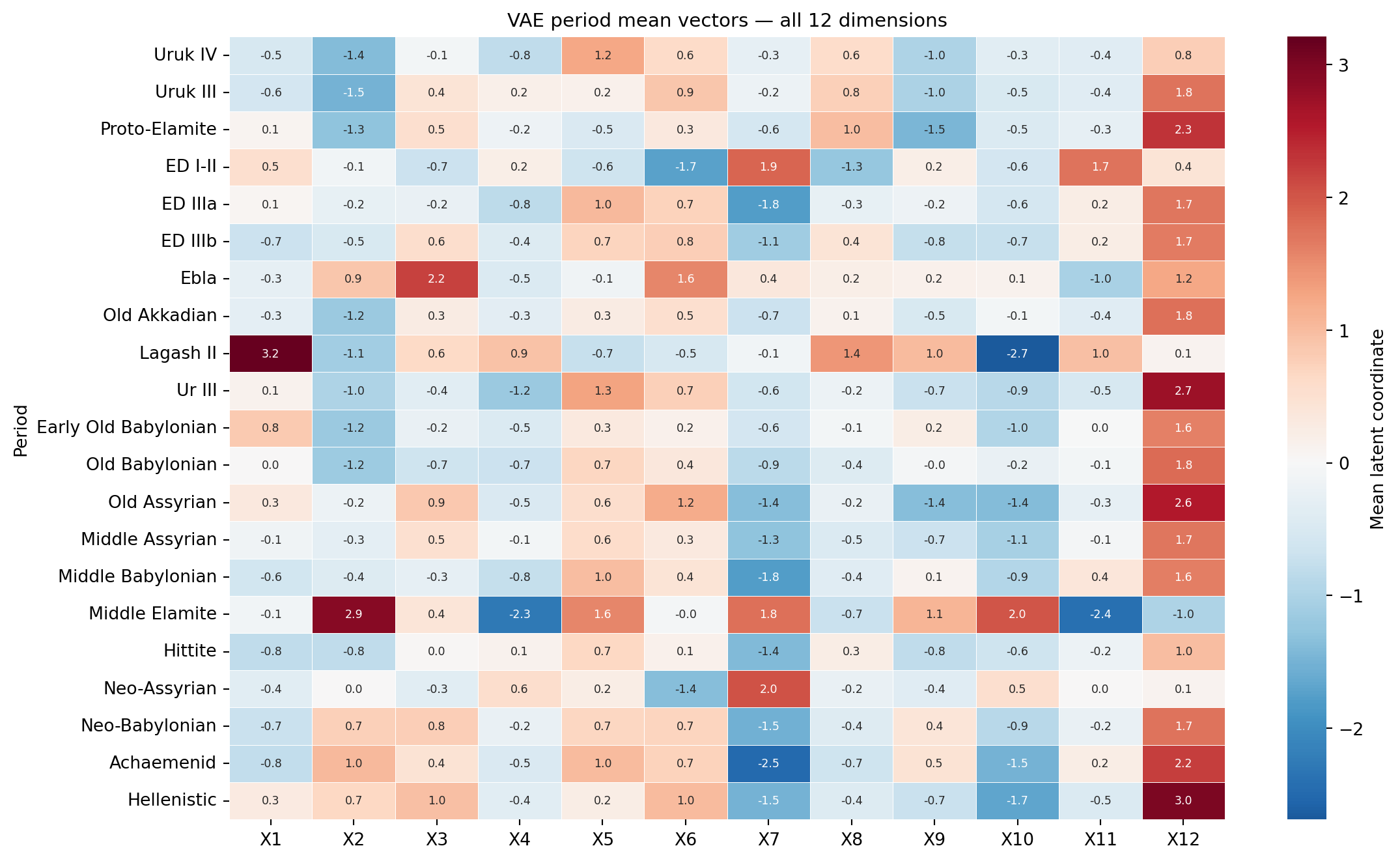
---title: "4 · VAE Latent Space Analysis"subtitle: "Interpretable shape features and diplomatic genealogies"sidebar: analyses---> **Paper section:** Results §3.3 · **Notebooks:** `2.4`, `10`, `10.1`, `11`, `11.1`## OverviewA Variational Autoencoder (VAE) with a 12-dimensional bottleneck compresses eachtablet's 80×80 binary silhouette into a structured 12-number vector. Unlike pixelratios or classification labels, these 12 coordinates form a **continuous geometricspace** in which similar tablet shapes cluster together and morphological transitionscan be traced as paths.Two key questions drive this analysis:1. Which dimensions best **discriminate between historical periods**?2. Which dimensions best **track the diachronic trend** across time?The answer to these questions is the same for no single dimension — and thatdissociation is itself the finding.## Discrimination vs. trend: the core result```{python}#| label: fig-eta2-rho#| fig-cap: "Kruskal-Wallis η² (period discrimination power, y-axis) vs. Spearman |ρ| (diachronic trend strength, x-axis) for all 12 VAE dimensions. Significant trend dimensions (p < 0.05) shown in red."import pandas as pd, matplotlib.pyplot as plt, numpy as npdf = pd.read_csv("../../paper/figures/vae_dim_stats.csv")fig, ax = plt.subplots(figsize=(7, 5))colors = ['#b5622e'if s =='**'else'#4a6fa5'for s in df['sig']]ax.scatter(df['abs_rho'], df['eta2'], c=colors, s=90, zorder=5, edgecolors='white', lw=0.8)for _, row in df.iterrows(): ax.annotate(row['Dimension'], (row['abs_rho'], row['eta2']), xytext=(5, 3), textcoords='offset points', fontsize=8)ax.axhline(0.06, color='grey', ls='--', lw=0.8, alpha=0.6)ax.axvline(0.45, color='grey', ls='--', lw=0.8, alpha=0.6)ax.set_xlabel("|Spearman ρ| — diachronic trend strength", fontsize=10)ax.set_ylabel("Kruskal-Wallis η² — period discrimination", fontsize=10)ax.set_title("VAE dimensions: discrimination vs. diachronic trend", fontsize=11)ax.text(0.02, 0.37, 'Strong discriminator\nno trend', fontsize=7, color='grey')ax.text(0.48, 0.04, 'Strong trend\nmodest discriminator', fontsize=7, color='#b5622e')plt.tight_layout()plt.show()``````{python}#| label: tbl-vae-stats#| tbl-cap: "Kruskal-Wallis η² and Spearman ρ for all 12 VAE dimensions."df_display = df[['Dimension','eta2','effect','rho','p','sig']].copy()df_display.columns = ['Dimension', 'η²', 'Effect', 'Spearman ρ', 'p', 'Sig.']df_display['η²'] = df_display['η²'].round(3)df_display['Spearman ρ'] = df_display['Spearman ρ'].round(3)df_display['p'] = df_display['p'].round(4)df_display.style \ .highlight_between(subset=['Spearman ρ'], left=0.5, right=1.0, color='#ffe0b2') \ .highlight_between(subset=['Spearman ρ'], left=-1.0, right=-0.5, color='#ffe0b2') \ .highlight_between(subset=['η²'], left=0.15, right=1.0, color='#e3f2fd')```## The two key dimensions**X7 — diplomatic-tradition axis** (η² = 0.435, best discriminator; ρ = −0.430, no trend)X7 separates scribal traditions by their characteristic portrait or landscape format,regardless of when those traditions were active:```{python}#| fig-cap: "Mean X7 value by period, sorted chronologically. High X7 = portrait tradition; low X7 = landscape tradition."import pandas as pd, matplotlib.pyplot as plt, numpy as npvae = pd.read_csv("../../paper/figures/vae_period_mean_vectors.csv")chron_order = ['Uruk IV','Uruk III','Proto-Elamite','ED I-II','ED IIIa','ED IIIb','Ebla','Old Akkadian','Lagash II','Ur III','Early Old Babylonian','Old Babylonian','Old Assyrian','Middle Assyrian','Middle Babylonian','Middle Elamite','Hittite','Neo-Assyrian','Neo-Babylonian','Achaemenid','Hellenistic']vae['_rank'] = vae['Period'].map({p: i for i, p inenumerate(chron_order)})vae = vae.sort_values('_rank')fig, ax = plt.subplots(figsize=(9, 4))colors = ['#c0392b'if v >0else'#2980b9'for v in vae['X7']]ax.bar(range(len(vae)), vae['X7'], color=colors, alpha=0.85, edgecolor='white', lw=0.5)ax.set_xticks(range(len(vae)))ax.set_xticklabels(vae['Period'], rotation=45, ha='right', fontsize=7.5)ax.axhline(0, color='black', lw=1)ax.set_ylabel('X7 mean (portrait ↑ / landscape ↓)', fontsize=9)ax.set_title('VAE X7 — diplomatic-tradition axis (non-monotonic)', fontsize=10)plt.tight_layout()plt.show()```**X2 — diachronic-drift axis** (ρ = +0.655, p = 0.001; η² = 0.078)X2 increases monotonically across time, tracking the combined portrait-to-landscaperotation and outline regularization:```{python}#| fig-cap: "Mean X2 value by period with Spearman trend line. X2 tracks the historical drift from complex portrait silhouettes to compact landscape forms."fig, ax = plt.subplots(figsize=(9, 4))ax.plot(range(len(vae)), vae['X2'], 'o-', color='#b5622e', lw=2, ms=6)from scipy.stats import spearmanr, linregressslope, intercept, _, _, _ = linregress(range(len(vae)), vae['X2'])ax.plot(range(len(vae)), [intercept + slope*i for i inrange(len(vae))],'--', color='#888', lw=1.5, label=f'Trend (ρ=+0.655, p=0.001)')ax.axhline(0, color='black', lw=0.8, ls=':')ax.set_xticks(range(len(vae)))ax.set_xticklabels(vae['Period'], rotation=45, ha='right', fontsize=7.5)ax.set_ylabel('X2 mean (increases → landscape+compact)', fontsize=9)ax.set_title('VAE X2 — diachronic-drift axis (monotonic trend)', fontsize=10)ax.legend(fontsize=9)plt.tight_layout()plt.show()```## Period mean vectors: full heatmap```{python}#| fig-cap: "Heatmap of mean VAE latent coordinates for all 21 periods × 12 dimensions. Colour scale: blue = negative, red = positive."import seaborn as snsvae_heat = vae.set_index('Period')[['X1','X2','X3','X4','X5','X6','X7','X8','X9','X10','X11','X12']]fig, ax = plt.subplots(figsize=(12, 7))sns.heatmap(vae_heat, center=0, cmap='RdBu_r', annot=True, fmt='.1f', annot_kws={'size': 6.5}, linewidths=0.3, cbar_kws={'label': 'Mean latent coordinate'}, ax=ax)ax.set_title('VAE period mean vectors — all 12 dimensions', fontsize=11)plt.tight_layout()plt.show()```## Diplomatic genealogies: hierarchical clusteringThe dendrogram of the 21 period mean vectors groups periods by shape similarity, not by date.Three historically meaningful clusters emerge:1. **Neo-Babylonian → Achaemenid → Hellenistic**: Late Babylonian institutional continuity2. **Ur III → Old Babylonian → Early OB**: Babylonian portrait tradition3. **Neo-Assyrian** as outlier: extreme portrait orientation (X7 = +2.05){#fig-dendrogram}::: {.callout-note}**Next:** [Shape Traversal →](05-traversal.qmd) — the physical meaning of X2, X7, and X8.:::